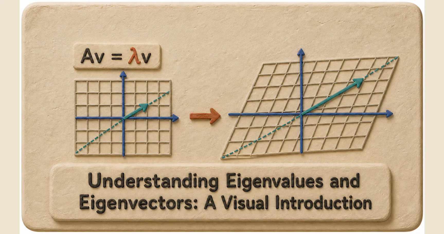
Understanding Eigenvalues and Eigenvectors: A Visual Introduction

Introduction

A matrix represents a linear transformation. In other words, a matrix represents a transformation that you apply to the vectors in your coordinate space.

Say, you apply the matrix:

A = \begin{bmatrix} 2 & 3 \\ 1 & 0 \end{bmatrix}

to a vector:

\vec{v} = \begin{bmatrix} 0 \\ 2 \end{bmatrix}

like this:

\begin{bmatrix} 2 & 3 \\ 1 & 0 \end{bmatrix}\begin{bmatrix} 0 \\ 2 \end{bmatrix} = \begin{bmatrix} 6 \\ 0 \end{bmatrix}

You will get a new vector:

A\vec{v} = \begin{bmatrix} 6 \\ 0 \end{bmatrix}

Again, a matrix represents a linear transformation that you apply to the vectors in a coordinate space. Because of this, all the vectors in the coordinate space get transformed into new vectors. As a result, the entire coordinate grid gets transformed.

Matrix transforming a vector and the coordinate grid

Diagram I: The matrix transforms both the vector and the coordinate grid.

Eigenvalues and Eigenvectors

Span of a Vector

Consider the vector v = (-3, 1). All the scalar multiples of this vector lie on the same line passing through the origin. This line is called the span of the vector.

\operatorname{span}(\vec{v})=\lbrace c\vec{v}\mid c\in\mathbb{R}\rbrace

The span of the vector v equals negative three comma one

The span of a nonzero vector in two-dimensional space is a line passing through the origin.

Eigenvector

When you multiply a matrix by a vector, the transformed vector may shift away from its original span; that is, its direction may change.

But there can be a few nonzero vectors that do not move away from their span after the transformation. Such vectors are called eigenvectors.

There can also be cases where the magnitude of the vector changes, but the vector remains in the same span. We can still say that it is an eigenvector.

For example, suppose a separate linear transformation T transforms the vector v = (2, 0) into Tv = (4, 0). Its magnitude is doubled, but it still lies on the same line.

The vector is scaled, but it remains in the same span.

Therefore, v = (2, 0) is an eigenvector of this transformation.

Eigenvalue

The scalar factor by which an eigenvector is scaled is called its eigenvalue.

In this example, the vector is scaled by 2. Hence, its eigenvalue is 2.

So, when a transformation represented by a matrix A is applied to an eigenvector v, the transformed vector becomes λv:

A\vec{v}=\lambda\vec{v},\qquad\vec{v}\neq\vec{0}

Here, λ is a scalar called the eigenvalue.

The eigenvalue is not the magnitude of the vector. It is the scaling factor. The magnitude of the vector changes by a factor of |λ|.

If λ > 0, the vector points in the same direction. If λ < 0, it points in the opposite direction. In both cases, it remains in the same span and is still an eigenvector.

If λ = 0, the vector is transformed into the zero vector. Zero can also be an eigenvalue.

In this example:

\lambda=2

Therefore, 2 is the eigenvalue.

Finding Eigenvalues and Eigenvectors

Now that we know what eigenvalues and eigenvectors are, let us see how to calculate them for a given matrix.

For this, consider a square matrix:

A\in\mathbb{R}^{n\times n}

Note: Eigenvalues and eigenvectors are defined only for square matrices.

Unlike SVD, we do not calculate AᵀA. We work directly with A.

The core calculation has two main parts. First, we find the possible values of λ. After that, we use each value of λ to find its corresponding eigenvector.

Form the Characteristic Equation

Start by subtracting λ from every diagonal element of A:

A-\lambda I

Here, I is the identity matrix of the same size as A.

For example, if

A=\begin{bmatrix}a & b \\ c & d\end{bmatrix}

then

A-\lambda I=\begin{bmatrix}a-\lambda & b \\ c & d-\lambda\end{bmatrix}

Now calculate the determinant and set it equal to zero. This gives us the characteristic equation:

\det(A-\lambda I)=0

For a 2 × 2 matrix, it becomes:

(a-\lambda)(d-\lambda)-bc=0

\lambda^2-(a+d)\lambda+(ad-bc)=0

Solve for the Eigenvalues

Now solve the characteristic equation for λ. The values of λ that satisfy this equation are the eigenvalues of A:

\lambda_1,\lambda_2,\ldots,\lambda_n

Depending on the matrix, an eigenvalue can be positive, negative, zero, repeated, or even complex.

Find the Corresponding Eigenvectors

For each eigenvalue λᵢ, substitute it into:

(A-\lambda_i I)\vec{v}_i=\vec{0}

Then solve the resulting system of linear equations.

The system will have at least one free variable. Assign convenient values to the free variables, making sure that the resulting vector is not zero, and calculate the remaining variables.

The resulting nonzero vector is an eigenvector:

\vec{v}_i=\begin{bmatrix}x_1 \\ x_2 \\ \vdots \\ x_n\end{bmatrix}

Note: The zero vector can never be an eigenvector.

Any nonzero scalar multiple of an eigenvector is also an eigenvector corresponding to the same eigenvalue.

Normalize the Eigenvectors if Required

Eigenvectors do not have to be unit vectors. Normalize an eigenvector only if the question asks for a unit eigenvector.

First, calculate its magnitude:

\left|\vec{v}_i\right|=\sqrt{x_1^2+x_2^2+\cdots+x_n^2}

Then divide the eigenvector by its magnitude:

\hat{v}_i=\frac{\vec{v}_i}{\left|\vec{v}_i\right|}

Verify the Result

Finally, check whether:

A\vec{v}_i=\lambda_i\vec{v}_i

If both sides are equal, the eigenvalue and eigenvector are correct.

Short Formula Sheet

\boxed{\det(A-\lambda I)=0}

This gives the eigenvalues.

For each eigenvalue, solve:

\boxed{(A-\lambda I)\vec{v}=\vec{0}}

This gives the corresponding eigenvectors.

Finally, verify:

\boxed{A\vec{v}=\lambda\vec{v}}

Special Case: Repeated Eigenvalues

If an eigenvalue occurs more than once, solve

(A-\lambda I)\vec{v}=\vec{0}

in the usual way and find all its linearly independent solutions.

A repeated eigenvalue may have fewer linearly independent eigenvectors than its algebraic multiplicity. Therefore, some matrices may not have enough independent eigenvectors to be diagonalized.

Conclusion

I hope this post made eigenvalues and eigenvectors a little easier to understand. If you have any questions, please leave a comment below. Thanks for reading 😊.